Last week I wrote an article about using a cluster computing system to generate a large amount of forecasts from time series data for the supply management units (SMU) in the Marine Corps. This system generated over four million time series forecasts for the SMUs, covering a period of eight calendar quarters from unit demand data throughout the Marine Corps.

Of course, once we generate the forecasts, we want to validate performance. This was made possible by constructing a simulation that we can plug the forecasts into, simulating the warehouses that we would stock and fill demands from. A “fill” is a demand that can be met directly from stocks. If the part has to be ordered from another agency because it isn’t in the warehouse, it isn’t considered a fill.

Two metrics were used to gauge fill rate. A “gross” fill rate: demands were filled by the SMU whether there was a demand history for the item or not. If there was a previous demand for the item, then we had the opportunity to build a forecast from it. If there was no previous demand, then there was no possibility to build a forecast.

In the simulation a fixed forecast that was based on the average quarterly demand (AQD) for items was used as a control case, against the forecasts generated with the cluster-computing/parallel core R software. For a synopsis of the 42 different time series analysis used for each history, see the article here.

Analysis of the results revealed that there was little difference between using the average quarterly demand as a forecasting tool, or the time series analysis forecast from the R solutions. Here are the results for gross fill rate for the three largest SMUs in the Marine Corps.

The results are inconclusive at best. The control method results are similar to the time series analysis forecasts, and the differences are within the margin of statistical error.

The second metric used, was the forecast fill rate. This is a measurement based on performance of the forecasts. If we had a demand history, and generated a forecast, how well did that forecast perform?

The results for forecast fill rate for the three main SMUs outlined the differences between using the time series method and a fixed average:

The time series analysis forecasts significantly outperformed the control group that used a fixed average.

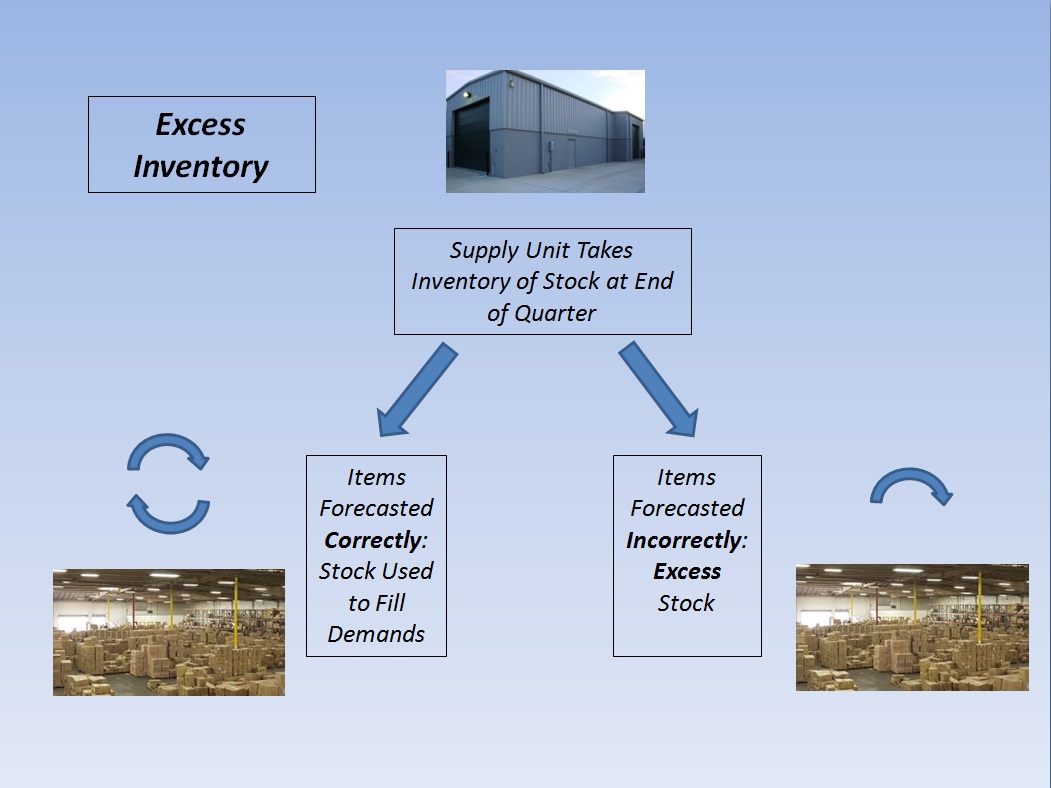
The third metric used was excess inventory. Excess inventory is defined as warehouse inventory that was forecast and not used. Excess inventory costs money to order, money to maintain, and clogs up the warehouse. The simulation counts inventory and reorders stock for the supply units at the end of each quarter. Time delays are used to simulated transport times to the SMUs.

Here is where the differences between using a fixed average and time series analysis start to really show.

And these are just the consumable parts cost, we’re not counting the transportation costs, warehousing costs, and disposal costs. If we look at the total savings over eight quarters we see:

Significant savings using a time series analysis forecasting method. Again, these are only the direct costs on purchasing the consumable items. The bottom line is, using a fixed average to stock your warehouse may be a quick way to accomplish the mission, but the costs of using that methodology are considerable.