The Hubble Tension May Be More Than One Number

For more than a decade, cosmologists have faced an uncomfortable problem: different ways of measuring the expansion of the universe don’t quite agree.

Measurements based on the nearby universe, particularly Cepheid-calibrated Type Ia supernovae, generally favor a present-day expansion rate near 73 kilometers per second per megaparsec. Measurements inferred from the cosmic microwave background, using the standard ΛCDM cosmological model, favor a value closer to 67–68. That disagreement is known as the Hubble tension.

Most discussions reduce it to a contest between two values of the Hubble constant, (H_0). Our new analysis asks a different question: What if the disagreement isn’t just a different value of (H_0)? What if the two approaches imply slightly different expansion histories as we look back through cosmic time?

The full paper and supporting material are publicly available here. I also built an interactive visualization of the result

What is the Hubble tension?

The Hubble constant tells us how quickly the universe is expanding today. A simple way to think about it is that a galaxy twice as far away should, on average, recede about twice as quickly. Edwin Hubble’s original discovery of this relationship eventually became the basis for measuring the cosmic expansion rate. But modern cosmology can estimate that rate in very different ways.

One approach starts nearby. Astronomers calibrate stellar distances, use those stars to calibrate supernovae, and then use supernovae to reach deeper into the universe. This is usually called the distance ladder. Another approach begins almost at the opposite end of cosmic history. The Planck satellite measured tiny temperature fluctuations in the cosmic microwave background, the afterglow of the early universe. Given a cosmological model, those measurements can be evolved forward to predict today’s expansion rate. The Hubble tension problem is that the answers remain different even as the measurements have improved.

That could mean several things: there may be an unknown systematic error, some part of the standard cosmological model may be incomplete, or some new piece of physics may be affecting the expansion history.

Instead of asking which (H_0) is right, we compared the histories

Our paper constructs three fixed expansion histories. The first, which we call R, represents the low-redshift distance-sector solution and has $H_0 \approx 72.8\ {\rm km,s^{-1},Mpc^{-1}}.$ The primary Planck-compatible reference, C1, has $H_0 \approx 68.0\ {\rm km,s^{-1},Mpc^{-1}},$ and a second Planck-compatible reference, C2, provides a check on how sensitive the result is to the exact CMB reference construction. The important result is that the difference between R and the Planck histories is not constant with redshift. If this were merely a disagreement about one calibration number, we would expect something much closer to a uniform shift. Instead, the difference changes shape as we look farther back in time.

In plain English: The expansion history favored by the distance data isn’t simply the Planck expansion history with a different number pasted onto the front. The gap between them changes with cosmic epoch. That is the central result of our findings.

There is a recognizable shape to the disagreement

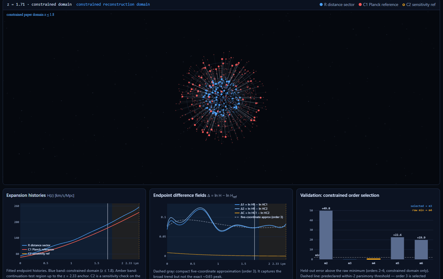
We define the difference approximately as $\Delta(z)=\ln H_R(z)-\ln H_{\rm CMB}(z).$ Over the portion of the data where the reconstruction is constrained, out to redshift $z\leq1.8,$ this difference forms a smooth structure rather than random wandering. Its largest amplitude occurs around $z\approx0.65.$ Even more interesting, replacing one Planck-compatible reference with the second hardly changes the overall pattern.

Across the constrained redshift bins, the difference between the two Planck references is only about 1% to 8% as large as the corresponding difference between the distance-sector history and the Planck references. The two distance-versus-CMB difference curves have a cosine similarity of about 0.9997, meaning that geometrically they point in almost exactly the same direction. The structure isn’t primarily being generated by some peculiarity of one particular Planck reference calculation.

The pattern is surprisingly compact

We also asked how complicated a mathematical description is needed to reproduce the difference. A very flexible model can obviously follow almost any curve, but that’s not very interesting. The useful question is whether a small number of degrees of freedom can describe the pattern and still work on data that were held back during fitting. A five-coordinate, order-3 representation did that job. A slightly more complicated order-4 model achieved the lowest raw validation score, but only by about 0.13 in $(\chi^2)$. Under our predeclared rule favoring the smallest model within two points of the best predictive score, the simpler order-3 reconstruction was selected.

That means the difference appears to be low-dimensional. It doesn’t require dozens of arbitrary wiggles to describe. This is one reason I think the result is interesting. If the discrepancy had required a wildly irregular function, the natural suspicion would be noise, overfitting, or complicated data systematics. Instead, the data seem to be describing a fairly coherent redshift-dependent structure.

There is also a scale difference

The distance-sector solution carries an effective acoustic ruler around $r_d\approx135.4\ {\rm Mpc}$, compared with roughly
$147.1\ {\rm Mpc}$ for the Planck-compatible references. That’s about an 8% difference. But the paper finds that a change in ruler scale alone doesn’t describe everything. There is also a shape difference with redshift. Many proposed solutions to the Hubble tension focus on shrinking the early-universe sound horizon. If all that was necessary were a uniform ruler change, the problem would be conceptually simpler. Our reconstruction suggests that whatever eventually explains this discrepancy may have to account for both scale and redshift-dependent shape.

The high-redshift test is also informative

There is one important boundary to the result: the compact reconstruction works over the constrained domain, $z\leq1.8$, but when it is simply extrapolated to the DESI Lyman-alpha measurement at z=2.33, that continuation fails. That tells us that the simple low-dimensional curve we’ve identified should not just be extended indefinitely toward the early universe. Whatever ultimately produces the effect may turn over, transition, or connect to high-redshift cosmology in a different way.

What the visualization is showing

The interactive simulation is designed to make the result intuitive rather than to depict the universe literally. Each pair of points represents the same synthetic galaxy tracer viewed through two different fitted expansion histories. The blue points represents the distance-sector history R. The red points represents the primary Planck-compatible reference C1. A line joins them, showing the difference in inferred radial position. Those lines are deliberately exaggerated, currently by a factor of eight, because the real differences would be difficult to see on a screen. The display itself states this explicitly. The simulation is not suggesting that galaxies actually occupy two locations or that the Big Bang was an explosion from the center of a sphere.

As the simulation evolves, the bright shell follows redshift while the graphs underneath show the corresponding expansion histories and their difference. The blue-shaded range marks the constrained reconstruction domain ($z\leq1.8$), while the higher-redshift region leads toward the separate Lyman-alpha continuation test.

The visualization also displays the model-selection result, the five-of-five projected Jacobian rank, the approximately 0.92 ruler ratio, and the failed (z=2.33) continuation test.

What physical process could produce this particular redshift-dependent difference in the expansion history?

Any proposed explanation can now be challenged to reproduce several features at once:

• a higher local expansion rate;
• an acoustic-ruler difference;
• a smooth redshift-dependent shape;
• a broad maximum in the difference around$(z\sim0.65)$;
• consistency with the low- and intermediate-redshift distance data;
• and some different behavior before the Lyman-alpha point at (z=2.33).

That is considerably harder than merely adjusting (H_0).

What could physically cause this?

There are several possibilities:

Evolving dark energy

The simplest conceptual possibility is that dark energy isn’t perfectly constant. In standard ΛCDM, dark energy behaves like a cosmological constant. Its density doesn’t evolve the way matter or radiation does. If the effective properties of dark energy change with time, however, they can alter (H(z)) differently at different redshifts. A smooth late-time change could potentially generate something resembling the reconstructed shape. The next question would then be whether such a model can reproduce the expansion history and remain consistent with structure formation, gravitational lensing and the CMB.

New early-universe physics

Another family of explanations changes conditions before or around recombination. If early-universe physics changes the sound horizon, it changes the standard ruler used by BAO and CMB analyses.This is the basic motivation behind early-dark-energy models and related proposals. Our result makes the problem more demanding, though, because the observed difference contains a redshift-dependent shape in addition to the ruler shift. A successful early-universe model may therefore need either to generate that later behavior naturally or work together with a second late-time effect.

A combination of early and late physics

This is an especially interesting possibility, there may be no single mechanism to carry the entire Hubble tension. One physical effect could slightly alter the early-universe acoustic ruler, while another modifies the later expansion history. That kind of hybrid explanation may ultimately be less extreme than trying to make one new field or interaction do everything.

Modified gravity

General relativity relates the energy content of the universe to its expansion. If gravity behaves somewhat differently on cosmological scales, the relationship between matter, dark energy and (H(z)) could change. The advantage of this possibility is that modified gravity generally makes additional predictions. It should affect how cosmic structure grows, how gravitational lensing behaves and potentially how gravitational waves propagate. Those measurements provide ways to test the idea independently.

Something systematic in the observations

New physics isn’t the only possibility. Supernova calibration, population evolution, BAO modeling, covariance assumptions, or some currently unidentified observational effect could generate part of the structure. That possibility should be tested just as aggressively as new cosmology. One powerful approach will be to reconstruct the same quantity using different supernova compilations, cosmic chronometers, gravitational-wave standard sirens, lensing, redshift-space distortions and time-delay distances. If the same shape keeps appearing through genuinely different observational channels, the new-physics interpretation becomes much harder to dismiss.

The next step

The next job is to see which physical theories can produce something like it and then freeze those theories before exposing them to independent observations. For example, suppose an evolving-dark-energy model can reproduce the reconstructed (H(z)). It should then make a prediction for the growth of structure. We can calculate that prediction before looking at redshift-space distortion measurements. If it fails, the model fails. The same logic applies to gravitational lensing, cosmic chronometers, standard sirens and time-delay lenses. That is a much stronger scientific test than continuing to add parameters until the original data fit.

A different way of looking at the Hubble tension

The Hubble tension is usually displayed as two error bars that don’t overlap enough. That’s useful, but it may be hiding structure. Our result suggests that the disagreement between the distance and CMB sides can be treated as a function of redshift, not merely as a disagreement over today’s value of the Hubble constant, a function that appears surprisingly coherent. Whether it ultimately turns out to be new cosmological physics, an unexpected combination of known effects, or a previously hidden observational systematic remains to be determined. But now there is a more specific target to explain.

Read the full paper on GitHub

Explore the interactive visualization